Jan 8, 2025 9 min read Python

How to augment data for financial analysis using VAE.

VAE are probabilistic generative models that encode and decode data and generate new data samples by capturing the underlying structure of the data in a lower-dimensional latent space.

💡

The following article was written after using a VAE to generate synthetic S&P data for a Failed Breakdown model testing.

GitHub: https://github.com/usmanlakhani/vae_synthetic_financial_data/tree/main

A Variational AutoEncoder (VAE) is a generative model that uses probability and statistics to create synthetic data. Synthetic data is useful in cases where analysis is being conducted on a small data set and we require MORE data points to ensure our analysis is correct.

💡

Generative models are a class of statistical models that learn the underlying probability distribution of a dataset. This allows them to generate new data instances that resemble the training data.

How does a VAE work?

Before understanding what VAE is, it's important to understand Standard Auto Encoders (AE).

Standard Auto Encoders.

A standard autoencoder is a neural network designed for unsupervised learning. Its primary goal is to learn efficient representations of input data, often for dimensionality reduction, feature extraction, or denoising.

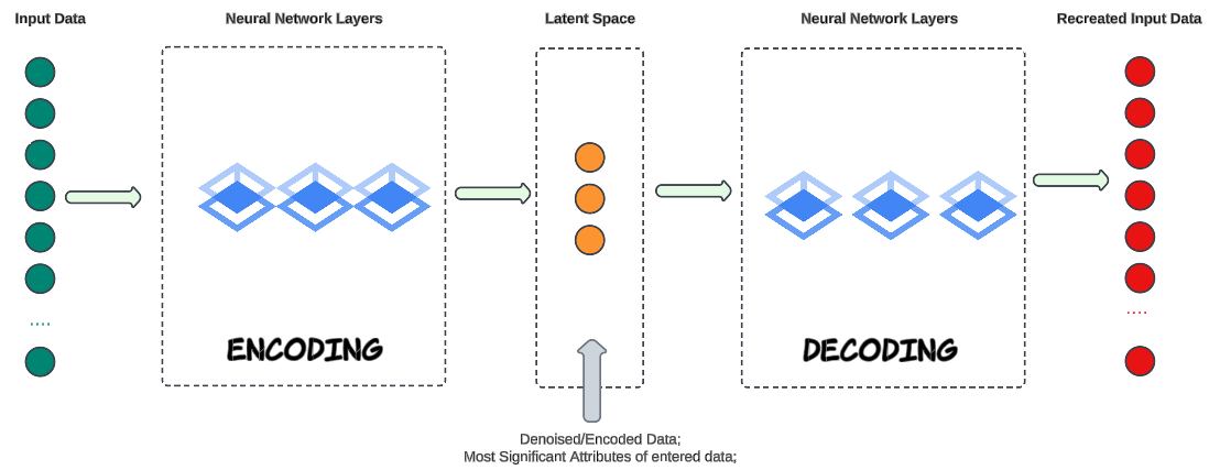
Encoding

Accepts input data (e.g. image, text, music etc).
Using Neural Networks, the input data 'core' attributes (data columns) are identified and marked (for future decoding purposes). These core attributes are saved in, what is called, a Latent Space (think of it as a box containing the core attributes we identified).
- Latent Space is also called the bottleneck. In our contemporary vernacular, a bottleneck is a fundamental "choke point" that creates a slowdown or blockage.

Decoding

Neural Networks will take the encoded data from the Latent Space and re-create the original input.

Training Process

Reconstruction Error: The autoencoder is trained by minimizing the difference between the original input and the reconstructed output. This difference is often measured using a loss function like mean squared error (MSE).

Backpropagation: The network learns by adjusting the weights of its connections through backpropagation, aiming to reduce the reconstruction error.

Expected Outcome with Standard AEs.

Standard AEs are deterministic and will attempt to recreate the original data from the encoded data saved in the Latent Space. While this is a great capability by itself, it does not generate new data points.

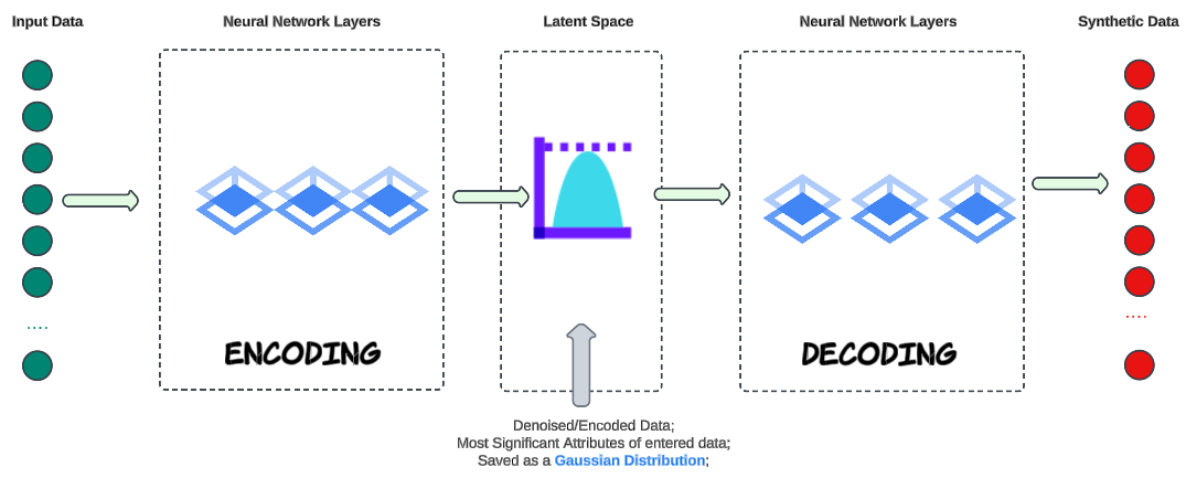
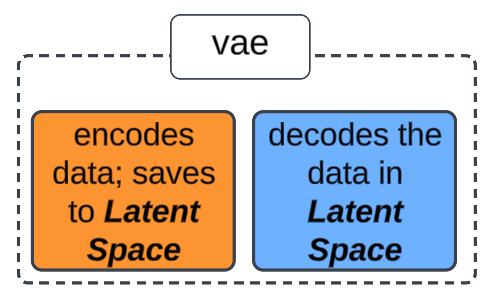
Enter VAE.

VAEs save encoded data as a distribution that has a mean, standard deviations and other statistics that can be used to generate multiple new data points as part of the encoding.

The **DECODER** will use the data distribution in the **Latent Space** and generate new synthetic data.

What is the reason for generating synthetic data that resembles the data you already have?

Data Augmentation.

Data Augmentation is a common technique used in machine learning to increase the diversity and size of the training dataset, helping improve the efficacy of machine learning models. Datasets may have missing values or incomplete records and a VAE can be used to impute such missing data points. By encoding the available data into the latent space, and then generating samples from the latent space, you can fill in missing values in a way that is consistent with the learned data distribution.

In Finance, VAEs can help create diverse sets of data for different scenarios, generating synthetic data that resembles historical or real-world data is essential for scenario analysis, risk assessment, and even investment strategies.

Demo Code.

💡

Python 3.12.8 was used for this demo.

Step 1: Import needed Python libraries.

import numpy as np
import tensorflow as tf
import matplotlib.pyplot as plt
import pandas_datareader as pdr

Step 2: Gather input data.

# Choose a start date and end date for our data gathering
sd = '2010-01-01'
ed = '2025-01-01'

# S&P 500 price data
data = np.array((pdr.get_data_fred('SP500', start=sd,end=ed)).dropna())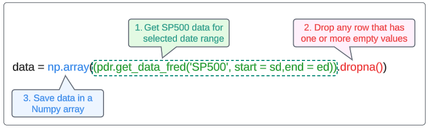

Step 3: Initiate the encoder.

latent_space_attributes = 2
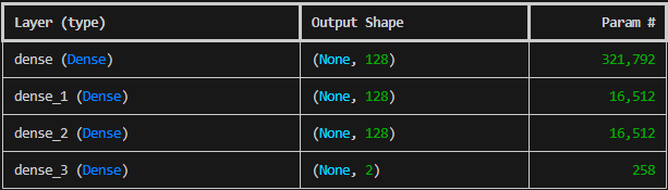
encoder = tf.keras.Sequential(
    [
        tf.keras.layers.Input(shape=(len(data),)),
        tf.keras.layers.Dense(128, activation='relu'),
        tf.keras.layers.Dense(128, activation='relu'),
        tf.keras.layers.Dense(128, activation='relu'),
        tf.keras.layers.Dense(latent_space_attributes, activation='relu'),
    ]
)

print (encoder.summary())

tf.keras.Sequential: The API in TensorFlow for creating simple neural networks.
tf.keras.layers.Input(shape=(len(data),)): Sets up the layer which will accept the data we downloaded in Step 2.
tf.keras.layers.Dense(128, activation='relu'): Sets up 3 layers, each with 128 neurons activated via ReLU (Rectified Linear Unit) activation function. ReLU is a common activation function that introduces non-linearity into the model.
tf.keras.layers.Dense(latent_space_attributes, activation='relu'): Represents the Latent Space (or bottleneck) layer.

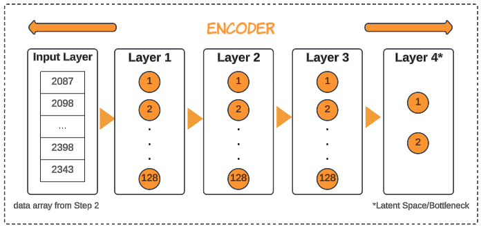
Visually speaking, Step 3 creates this learning architecture for the **ENCODER**.

Finally, the encoder.summary() call can be used to confirm the architecture in the code resembles the image above.

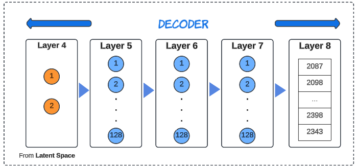
**encoder.summary()** will display a table, that looks like the above, in terminal.

Step 4: Configure the decoder.

decoder = tf.keras.Sequential([
    tf.keras.layers.Input(shape=(latent_space_attributes,)),
    tf.keras.layers.Dense(128, activation='relu'),
    tf.keras.layers.Dense(128, activation='relu'),
    tf.keras.layers.Dense(128, activation='relu'),    
    tf.keras.layers.Dense(len(data), activation='linear'),
])

The decoder will do the exact opposite of the encoder, by using the 'representation' of the data saved in the Latent Space layer and re-generate the encoded data points.

Visually speaking, Step 4 creates this learning architecture for the **DECODER**.

Step 5: Wire up the VAE model.

vae = tf.keras.Model(encoder.inputs, decoder(encoder.outputs))

This line scaffolds a VAE model, informing it of the inputs to train on while encoding and decoding.

Step 6: Compile the model.

vae.compile(optimizer = 'adam', loss = 'mse')

vae.compile: A Keras function that configures the model's learning process.
optimizer='adam': Sets the optimized algorithm to Adaptive Moment Estimation, a popular deep learning optimizer.
loss='mse': Sets the loss function to Mean Squared Error (MSE), which calculates the average squared difference between a prediction and its corresponding actual value.

At this point, the vae model has been created and compiled. It's now a matter of passing input data to it.

Step 7: Normalize the input data array.

normalized_data = (data - np.min(data)) / (np.max(data) - np.min(data))
normalized_data = normalized_data.reshape(1, -1)

Normalization is a typical pre-processing step and converts input data into a shape that is expected by TensorFlow.

Step 8: Train the model.

vae.fit(normalized_data, normalized_data, epochs = 1000, verbose = 0)

vae.fit: The Keras function that trains the model. It takes the training data, target values, and various other parameters to control the training process.
normalized_data, normalized_data: Specifies the input data and target values for training. In the case of an autoencoder, both the input and target are the same (normalized_data).
epochs=1000: Sets the number of epochs, which is one complete pass through the entire dataset, to 1000. Training for 1000 epochs means the model will see and learn from the entire dataset 1000 times.
verbose=0: Controls the amount of output displayed during training. verbose=0 means no output will be shown in the console.

What happens during training:

Forward Pass: The input data (normalized_data) is fed to the encoder, which compresses it into a Latent Space representation. This representation is then passed to the decoder, which tries to reconstruct the original input.
Loss Calculation: The loss function, set to Mean Standard Error (MSE), calculates the difference between the reconstructed output and the original input (normalized_data).
Backpropagation: The optimizer ('adam') uses the calculated loss to adjust the weights of the encoder and decoder networks. This adjustment aims to minimize the reconstruction error in the next forward pass.

These 3 steps are completed 1000 times (determined by the value provided for the number of epochs).

💡

Depending upon the number of epochs and, primarily, the strength of the CPU, model training may take upto 2 mins.

Step 9: Test the model.

The proof of the pie is in its eating, of course, and we should now be able to create synthetic data from our model.

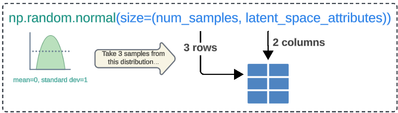
Step 9a: Create a 3x2 numpy array.

num_samples = 3
random_latent_vectors = np.random.normal(size=(num_samples, latent_space_attributes))

np.random.normal: A Numpy function that generates random numbers from a standard normal distribution with a mean of 0 and a standard deviation of 1.
size=num_samples,latent_space_attributes: An argument passed to np.random.normal for the number of rows and columns for the resulting array.
- Recall we had set the number of dimensions for our Latent Space to 2 (which is now being used to create the number of columns in our data array).

In one line of code, we will have created an array with 3 rows and 2 columns, and fill it with a set of random numbers from a normal distribution with **mean = 0** and **standard deviation = 1.**

Step 9b: Generate synthetic data.

decoded_data = decoder.predict(random_latent_vectors)

# Denormalize
decoded_data = decoded_data * (np.max(data) - np.min(data)) + np.min(data)

The vector created in Step 9a holds a normalized form of data that will be decoded and de-normalized.

💡

Why are we de-normalizing the decoded output?
Recall we had to normalize our input array in Step 7 for performance and API-specific needs and now we have to do the opposite to get useable 'real' outputs from our model.

Step 10: Visualize the results.

fig, axs = plt.subplots(2, 1)
axs[0].plot(data, label = 'Original Data', color = 'black')
axs[0].legend()
axs[0].grid()
for i in range(num_samples):
    plt.plot(decoded_data[i], label = f'Synthetic Generated Data {i+1}', 
             linewidth = 1)
plt.xlabel('Time Steps')
plt.ylabel('Value')
plt.legend()
plt.title('Original (black) vs. Synthetic Generated Time Series Data (colored)')
plt.show()
plt.grid()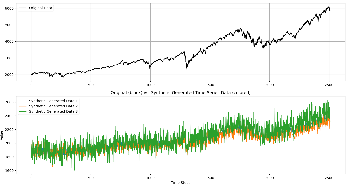

This technique can be used to generate and back test as much data as one needs for their models.

Complete Code

# Step 1: Import needed Python libraries.
import numpy as np
import tensorflow as tf
import matplotlib.pyplot as plt
import pandas_datareader as pdr
import sys

def initiate(startDate, endDate, latSpaceAttributes,ep,numSamples):

    # Step 2: Gather input data.
    #start_date = '2010-01-01'
    start_date = startDate
    #end_date   = '2025-01-01'
    end_date = endDate

    data = np.array((pdr.get_data_fred('SP500', start = start_date, end = end_date)).dropna())

    # Step 3: Initiate the encoder.
    latent_space_attributes = int(latSpaceAttributes)

    encoder = tf.keras.Sequential(
        [
            tf.keras.layers.Input(shape=(len(data),)),
            tf.keras.layers.Dense(128, activation='relu'),
            tf.keras.layers.Dense(128, activation='relu'),
            tf.keras.layers.Dense(128, activation='relu'),
            tf.keras.layers.Dense(latent_space_attributes, activation='relu'),
        ]
    )

    # Step 4: Configure the decoder.
    decoder = tf.keras.Sequential([
        tf.keras.layers.Input(shape=(latent_space_attributes,)),
        tf.keras.layers.Dense(128, activation='relu'),
        tf.keras.layers.Dense(128, activation='relu'),
        tf.keras.layers.Dense(128, activation='relu'),    
        tf.keras.layers.Dense(len(data), activation='linear'),
    ])

    # Step 5: Wire up the VAE model.
    vae = tf.keras.Model(encoder.inputs, decoder(encoder.outputs))

    # Step 6: Compile the model.
    vae.compile(optimizer = 'adam', loss = 'mse')

    # Step 7: Normalize the input data array.
    normalized_data = (data - np.min(data)) / (np.max(data) - np.min(data))
    normalized_data = normalized_data.reshape(1, -1)

    # Step 8: Train the model.
    history = vae.fit(normalized_data, normalized_data, epochs = int(ep), verbose = 2)

    # Step 9: Test the model.
    # Step 9a: Create a numpy array that will hold 3 rows and 2 columns of data
    num_samples = int(numSamples)
    random_latent_vectors = np.random.normal(size=(num_samples, latent_space_attributes))

    # Step 9b: Generate synthetic data
    decoded_data = decoder.predict(random_latent_vectors)
    decoded_data = decoded_data * (np.max(data) - np.min(data)) + np.min(data)

    # Step 10: Visualize the results.
    fig, axs = plt.subplots(2, 1)
    axs[0].plot(data, label = 'Original Data', color = 'black')
    axs[0].legend()
    axs[0].grid()
    for i in range(num_samples):
        plt.plot(decoded_data[i], label = f'Synthetic Generated Data {i+1}', 
                linewidth = 1)
    plt.xlabel('Time Steps')
    plt.ylabel('Value')
    plt.legend()
    plt.title('Original (black) vs. Synthetic Generated Time Series Data (colored)')
    plt.show()
    plt.grid()

if __name__ == "__main__":
    
    startDate = sys.argv[1]
    endDate = sys.argv[2]
    latSpaceAttributes = sys.argv[3]
    ep = sys.argv[4]
    numSamples = sys.argv[5]
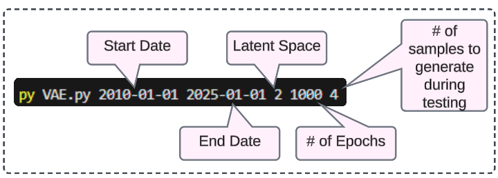
    initiate(startDate, endDate, latSpaceAttributes,ep,numSamples)

Execution Instructions

Save the python code as VAE.py (or a name of your choice) and pass the 5 inputs as shown in the image below.

I write to remember, and if, in the process, I can help someone learn about Containers, Orchestration (Docker Compose, Kubernetes), GitOps, DevSecOps, VR/AR, Architecture, and Data Management, that is just icing on the cake.