DS w/ P: Data Exploration and Cleaning.

Pre-Requisites: Primary

• We will use Python and Jupyter Notebooks for this article. Use this link to download the Anaconda terminal.
• The Default of Credit Card Clients data set from UCI Machine Learning Repository [http://archive.ics.uci.edu/ml]
  • The dataset has been tweaked to fit for purpose.

Step 1: After launching a Jupyter Notebook...

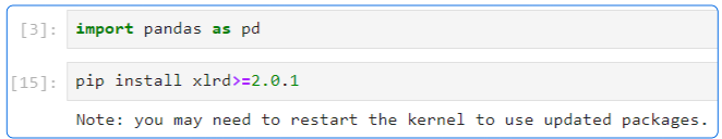
Step 2: Load the Excel sheet into the notebook

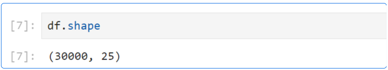
Step 3: Confirm the shape of the data loaded (df.shape)

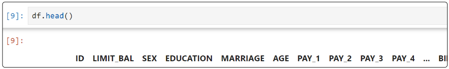
Step 4: Take a look at the columns (df.head())

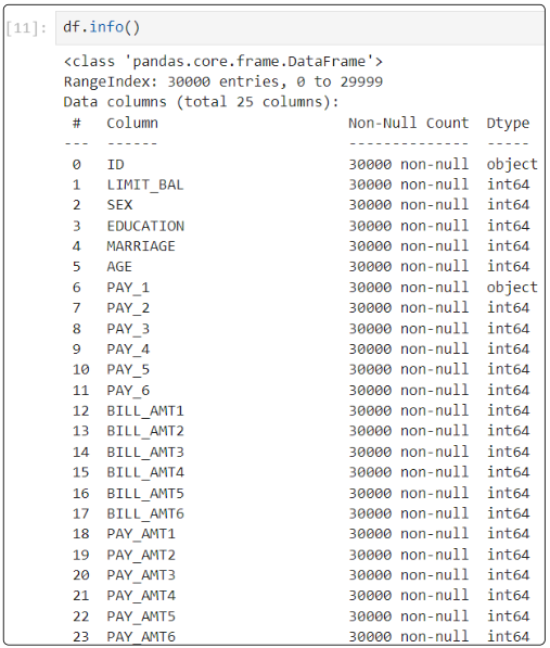
Step 5: Display the metadata in the data set (df.info())

So far, we have not discussed the question we hope to answer. Let's do that now before we proceed further.

So what is the business question that needs answering?

We must develop a predictive model based on a user's demographic and other historical data to determine if the user will default on their payment in the coming month.

Step 6: Let's do some Exploratory Data Analysis (EDA)

Usually, EDA can be difficult. If one knows the nature of the data, we can hypothesize and start our exploration, otherwise, it can be tricky.

We assume in our hypothetical case, we know only one fact about the data set:

All records have a unique ID

Is that true?

Let's investigate.

Start with df.column to print just the names of the columns.

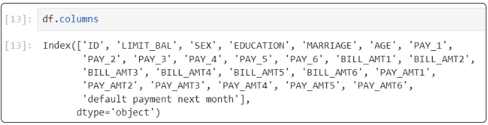
The data dictionary mapped to each column is below:

• ID: A unique identifier for each row in the data set
• LIMIT_BAL: The total credit amount available for a user/account
• SEX: Gender
  • 1 = male
  • 2 = female
• EDUCATION:
  • 1 = graduate school
  • 2 = university
  • 3 = high school
  • 4 = others
• MARRIAGE:
  • 1 = married
  • 2 = single
  • 3 = others
• AGE: in years
• PAY_1 to PAY_6: Record of past 6 monthly payments
  • -1 = pay duly
  • 1=payment delayed by a month
  • 2=payment delayed by 2 months and
  • continues to 9 (to indicate payment has been missed for 9 months)
• BILL_AMT1–BILL_AMT6: Bill statement amount corresponding to each PAY_# period
• PAY_AMT1–PAY_AMT6: Amount of previous payments, corresponding to PAY_# and BILL_AMT#

Step 7: Is the unique identifier (from the ID column) truly unique?

Is it? We can find out using unique().

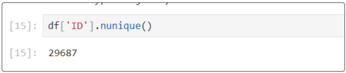
Its clear. All rows in the data frame DO NOT have unique IDs because if that were true, we would see 30000 instead of 29687.

Step 8: Which IDs are not unique?

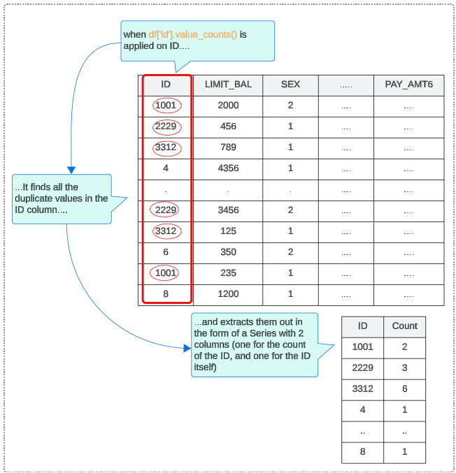
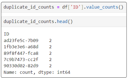
For this, use the value_count function (which is very much like SQL's Group By clause). This function extracts a series from the data frame and saves it to a variable.

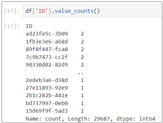
You can use the .head() method to display the first 5 records from the Series.

The resulting display of duplicate_id_counts will:

• Be in descending order such that the first element is the most frequently occurring element
• Excludes NA values by default

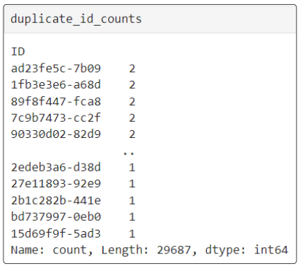
Since we know that the Series is arranged from the highest frequency of duplicate IDs to the lowest, the image above confirms that no ID repeats more than twice.

At this point, we know the following facts about our dataset:

1. It has 30,000 records
2. It has 25 columns
3. It has an ID column (being used for uniqueness)
4. There are ID values that are duplicates
5. At most, an ID has been duplicated only 2 times (which means that there are NO IDs that have been duplicated 3 times or more)

In the spirit of EDA, and data cleaning, let's continue to investigate the nature of the record that shares the same ID with another record.

Step 9: Distinguish the Unique IDs from the repeated ones using a Boolean Mask

We have a Series that contains the Unique IDs in one column and the number of times they are repeated in the second column.

To easily find WHICH of the IDs are duplicates (until now, we were just concerned with HOW many), we use a Boolean Mask.

The following is an example of a Boolean Mask

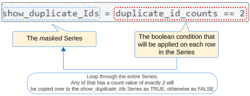
Think of the Boolean Mask as a filter. When it's applied to the duplicate_id_counts Series, it will:

1. Loop through the Series
2. Find all entries in the Series where the count value is exactly 2
   1. Copy them over into the show_duplicate_Ids (which is also a Series) but instead of saving the numeric count, it will save a True
3. Find all entries in the Series where the count value is 1
   1. Copy them over to the show_duplicate_Ids but save their value as False

Once the Boolean Mask is applied, we can display the contents of show_duplicate_Ids and notice ...

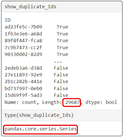
Since the Boolean Mask does not REMOVE any items in the collection, the resulting items are the same size as the collection that was masked.

Step 10: Separate the True (i.e. records with duplicated IDs) from the False (i.e. records with a unique ID)

We applied Boolean Mask on the original data frame, and now have a Series object that contains 29687 items with each either True (is duplicate) or False (is unique). So far so good. However, just labelling the records True or False is not particularly helpful. As part of our EDA and data cleaning, we should discover what is special about records that share an ID.

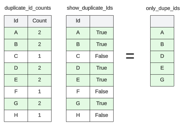
Panda uses the index attribute and a Boolean Mask, to take out all records with duplicate IDs and save them separately in a variable called only_dupe_ids.

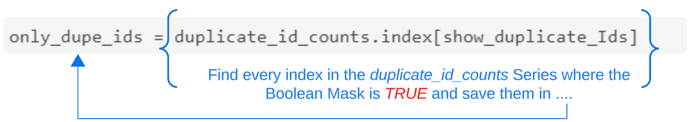
The .index attribute finds all Trues in the show_duplicate_Ids and copies them to only_dupe_ids.

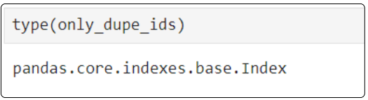
The type for only_dupe_ids is Pandas.Core.Indexes.base.Index.

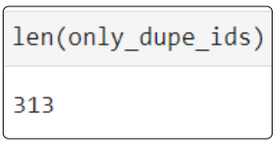
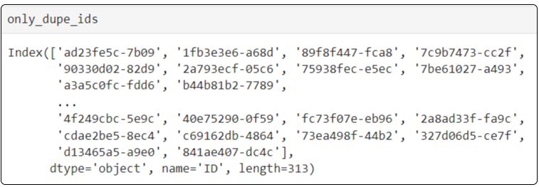
We can confirm that only_dupe_ids has 313 items since we know that out of the 30000 records, 29687 are not sharing IDs leaving 313 that are.

At this point, list the contents of only_dupe_ids.

Step 11: Isolate the raw records in the original data frame where IDs are shared (i.e not unique, >2)

Using Series and Index, we found out about non-unique IDs in the dataset.

The next step is to investigate these rows and understand if there is something unusual about them.

Finding the details associated with entries in the only_dupe_ids index is possible using isin and loc methods.

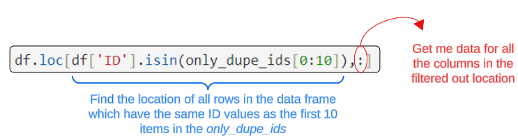
Executing this command will list data from the data frame we loaded all that while back (towards the start of this article).

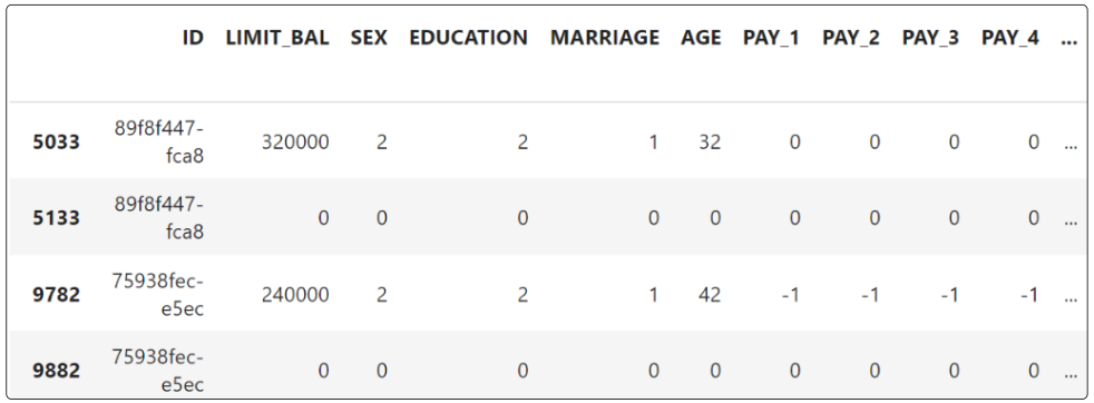
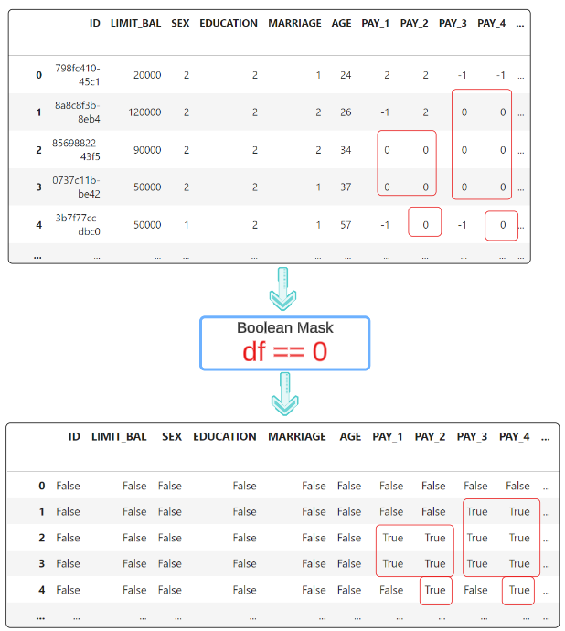
Notice that, in both sets in the image, one of the records has ZERO under the columns (barring the ID of course).

Aha! Our data cleaning and EDA efforts have shown us something important. We can remove one record from every duplicate set because having ZERO's for all other predictors provides no value for our investigation.

Step 12: Remove rows which have all ZEROs as column values

A rule of thumb is to always perform EDA against the original data source but when it comes to cleaning them, do that on a copy.

Since we are now at the stage where we have to clean the data frame (i.e. rid it of records with all features set to 0), we will be cautious and tread carefully.

Let's copy the original data frame and apply a Boolean Mask to it.

The resulting data frame (called df_w_True_False) looks like below.

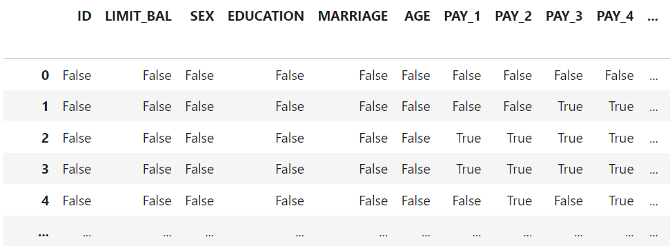
The Boolean Mask shows True wherever a 0 was found.

We want to loop through the df_w_True_False data frame, saving the index of records where all feature values are 0 and then removing them from the copied data set.

The easiest way to do this is through the use of a list.

The above can be read as:

"Save the index of ANY row in the df_w_True_False data frame where all features (apart from the ID) are Zero".

At this point, we have the indexes for all records in the df_w_True_False data frame with all 0's.

It is now simply a matter of using this list of indexes and deleting the erroneous data.

2 things are happening here:

• Using the all_rows_where_all_zero along with the ~ will isolate all rows where all values are NOT 0 and
• Copy them into a final and cleaned-up data frame we call df_cleaned.

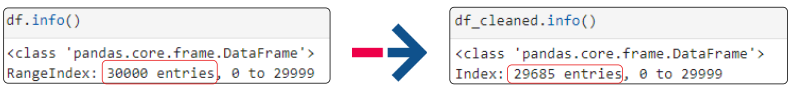
Step 13: Confirm df_cleaned is actually clean

Use df_cleaned.info() and you should see it has 29685 rows, down from the original 30000

Further Assessment for Data Quality.

Arduous as it was, we made it. The notion that every ID is unique was dispelled, courtesy Python but just because we have not been told about other problems, doesn't mean they don't exist.

Here is the tricky part of EDA. How do we make sure that other elements are in a clean state?

Since we don't know about anything else but the ID, we have to take a macro-view of the entire clean data set.

Step 14: Conduct a holistic assessment of the clean dataset

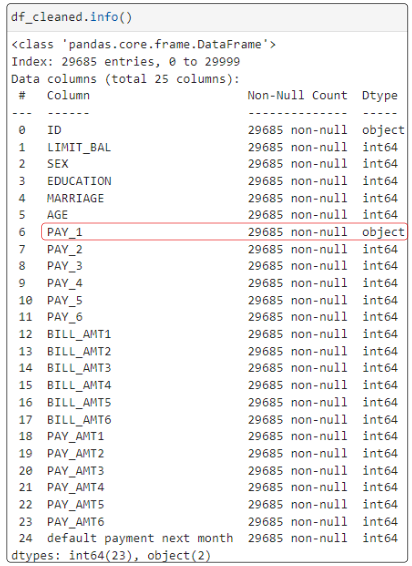
PAY_1 is off the reservation! Why? How?

Step 15: What's up with PAY_1?

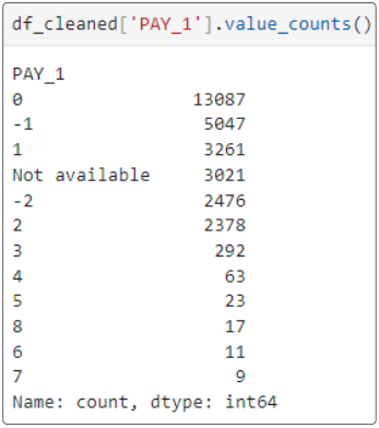
We now know of at least one other data element that has problems.

We will attempt to fix this issue in later articles. For now, let's delete any record where PAY_1 is 'Not available'.

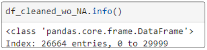
Finally, confirm df_cleaned_wo_NA is smaller in size than df_cleaned.

I write to remember, and if, in the process, I can help someone learn about Containers, Orchestration (Docker Compose, Kubernetes), GitOps, DevSecOps, VR/AR, Architecture, and Data Management, that is just icing on the cake.